Discrete Choice Models of Assortative Mating, Part 1: Simulating a Marriage Market

The first in a series looking at the advantages and pitfalls of using DCM for AM research. This post develops a simulated data set, and data generating functions, to be used in subsequent posts.

Introduction

There’s a been a subtle trend in sociological research on assortative mating away from log-linear modeling and towards a more flexible style of discrete choice modeling, primarily based on McFadden’s conditional logit model (1974).¹ Examples include the work of Karen Haandrikman (2012), Aaron Gullickson (2021), and my colleague and student, Jesper Lindmarker (2025). That this trend in assortative mating research is taking place outside of economics, where discrete choice models were first developed, is perhaps not too surprising: sociologists are less constrained by questions of causal identification, general equilibrium, and stable matching that often preoccupy economists. Using an out-of-the-box discrete choice modeling approach largely elides these issues in favor of arriving at parameter estimates that are causally/structurally ambiguous, but provide richer fodder for sociological interpretation.

But something that I think remains underappreciated is that the conditional logit model provides a more general formulation of the log-linear models that have served as the bread and butter of mobility and assortative mating research. In other words, you can use the conditional logit model to obtain identical parameter estimates and standard errors as equivalently specified log-linear models. This knowledge is not really new: Richard Breen (1994) has shown this, as has John A. Logan (1983). And Logan even points to knowledge of the equivalence dating back to the 1970s. Beyond producing parameter estimates that are identical to those produced using log-linear models for count data, Logan and Breen make the point that conditional logit models allow for the inclusion of idiosyncratic individual- and match-level covariates that more closely align with the theorizing and claims-making that sociologists and demographers are most interested in.

So a goal of these posts is to set down an accessible marker for future researchers seeking to integrate these models into their analytic practice, perhaps as an alternative or supplement to traditional log-linear modeling. Beyond that, I also want to explore the greater possibilities, as well as the interpretive perils, that go along with this modeling approach. I do so using a simulated dataset representing some stylized but essential features of assortative mating and marriage markets.

This is just part one in a series. I won’t make it to model fitting here. This post just sets the scene using simulation, stipulating and then allocating singles to social and spatial positions in a stylized marriage market and then forming unions between those singles using an econometric matching algorithm. In subsequent posts, I’ll show how to fit log-linear and conditional logistic regression models to the resulting data, how the parameter estimates compare, and then how these parameter estimates might give us a skewed view of the “deeper” parameters that may drive union formation in simulated and, of course, real-world data sets. So, let’s get to it.

Generating the marriage market

I consider a marriage market characterized by a simplified geographic space, consisting of spatial positions that are occupied by actors with a narrow set of attributes. I do this in three steps: first, I construct a grid of positions, then I generate a set of singles, and third I match singles to positions on the grid in such a way as to produce some spatial segregration.

Positions

I start with a square grid of discrete spatial locations for singles to occupy. I inflate the number of places in the grid so that there are some vacancies, i.e., there are more positions than there will be singles.

library(dplyr)
library(tidyr)
library(ggplot2)

make_locations <- function(n, relax = 1.2) {
  dim <- ceiling(relax * sqrt(n))
  expand_grid(
    x = (seq_len(dim) - .5) / dim,
    y = (seq_len(dim) - .5) / dim
  ) |>
    arrange(x, y) |>
    mutate(id_location = row_number()) |>
    select(id_location, x, y)
}
set.seed(543)
locations <- make_locations(n = 1000)
locations

# A tibble: 1,444 × 3
   id_location      x      y
         <int>  <dbl>  <dbl>
 1           1 0.0132 0.0132
 2           2 0.0132 0.0395
 3           3 0.0132 0.0658
 4           4 0.0132 0.0921
 5           5 0.0132 0.118 
 6           6 0.0132 0.145 
 7           7 0.0132 0.171 
 8           8 0.0132 0.197 
 9           9 0.0132 0.224 
10          10 0.0132 0.25  
# ℹ 1,434 more rows

Actors

I assume actors are split into two genders, men and women, with sebsequent unions constituted by opposite gendered pairs. I’ll make the market gender balanced for the sake of simplicity, and when all is said and done, each actor will be paired with one and only one opposite gender partner. Beyond gender and (eventually) position, I stipulate that each actor is characterized by just two other attributes: group membership, proxying something like race or ethnicity, and age, with the possibility of different age distributions for each group.

I use scaled beta distributions to generate the ages. This allows me to constrain the ages to fall between two bounds. This is represented in the following function:

rbeta_scaled <- function(n, mean, precision, min_value = 0, max_value = 1) {
  scaled_mean <- (mean - min_value) / (max_value - min_value)
  shape1 <- scaled_mean * precision
  shape2 <- (1 - scaled_mean) * precision
  min_value + (max_value - min_value) * rbeta(n, shape1, shape2)
}

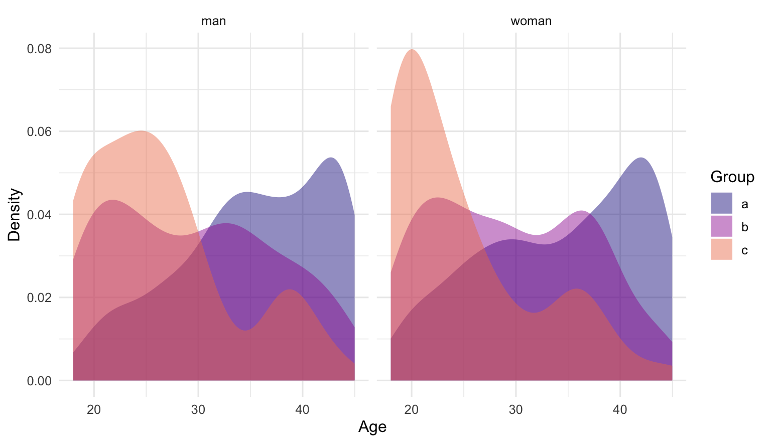
With this function in hand, I can create a dataset of simulated actors, for whom I also generate identifiers, which will be convenient in subsequent posts. The mean ages of the groups differ, but the age ranges are the same.

make_actors <- function(
  n,
  groups,
  group_shares,
  age_mean,
  age_min,
  age_max,
  age_concentration
) {
  G <- length(groups)
  group_shares <- group_shares / sum(group_shares)
  group_counts <- as.integer(n * group_shares)
  group_counts[G] <- n - sum(group_counts[-G])

  tibble(group = groups, age_mean, group_counts) |>
    reframe(
      age = rbeta_scaled(
        group_counts,
        age_mean,
        precision = age_concentration,
        min_value = age_min,
        max_value = age_max
      ),
      .by = c(group, age_mean)
    ) |>
    mutate(id = row_number()) |>
    group_by(group) |>
    mutate(sex = if_else(as.logical(row_number() %% 2), "man", "woman")) |>
    ungroup() |>
    select(id, sex, group, age)
}
actors <- make_actors(
  n = 1000,
  groups = c("a", "b", "c"),
  group_shares = c(60, 30, 10),
  age_mean = c(35, 30, 25),
  age_min = 18,
  age_max = 45,
  age_concentration = 2
)

slice_sample(actors, n = 10)

# A tibble: 10 × 4
      id sex   group   age
   <int> <chr> <chr> <dbl>
 1   996 woman c      18.0
 2   631 man   b      33.9
 3   575 man   a      44.3
 4    50 woman a      41.4
 5   685 man   b      24.0
 6   228 woman a      37.3
 7   939 man   c      37.8
 8    39 man   a      43.7
 9   146 woman a      29.7
10   834 woman b      21.2

The differing sampled age distributions, broken down separately for men and women, can be visualized using a density plot:

group_colors <- viridis::plasma(4)[1:3]
ggplot(actors, aes(age, fill = group)) +
  geom_density(alpha = 0.45, color = NA) +
  facet_wrap(~sex) +
  scale_fill_manual(values = group_colors) +
  labs(x = "Age", y = "Density", fill = "Group") +
  theme_minimal(base_size = 12)

Groups differ in mean age, but the simulated age distributions overlap.

Assigning actors to locations

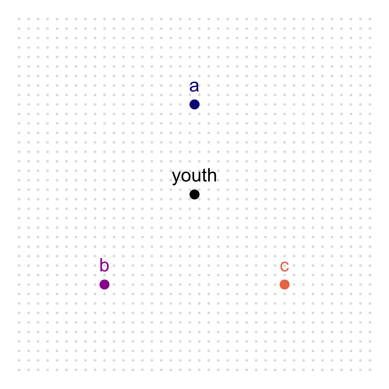
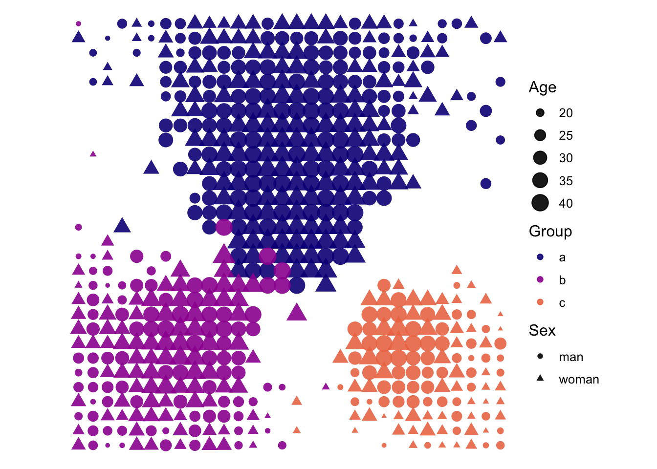
I want to introduce some group and age segregation into the simulated marriage market. I accomplish this by designating a set of poles that serve as attraction points. A point in the center pulls in younger actors. Then a set of three, group-specific poles outside the center pull in members of the corresponding group.

poles <- tibble(
  pole = c("a", "b", "c", "youth"),
  x_pole = c(0.5, 0.25, 0.75, 0.5),
  y_pole = c(0.75, 0.25, 0.25, 0.5)
)

ggplot() +
  geom_point(
    data = locations,
    aes(x, y),
    size = 0.8,
    alpha = 0.28,
    color = "#9aa0a3"
  ) +
  geom_point(
    data = poles,
    aes(x_pole, y_pole, color = pole),
    size = 5
  ) +
  geom_text(
    data = poles,
    aes(x_pole, y_pole, label = pole, color = pole),
    nudge_y = 0.055,
    size = 8,
    show.legend = FALSE
  ) +
  coord_equal() +
  scale_color_manual(values = c(group_colors, "black")) +
  labs(
    x = "Spatial coordinate x",
    y = "Spatial coordinate y"
  ) +
  theme_void(base_size = 12) +
  theme(
    legend.position = "none",
    plot.margin = margin(2, 2, 2, 2)
  )

Group-specific attractors and the central youth attractor.

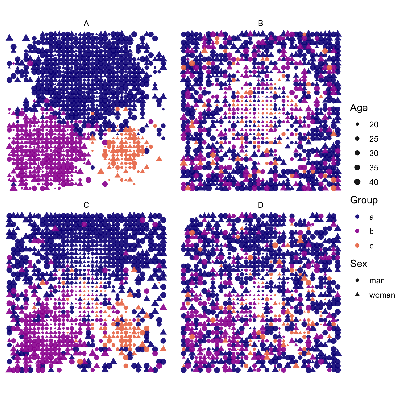
To assign actors to locations, I use a utility-based probabilistic assignment approach. The utility functin has deterministic and random parts. The deterministic part is a function of the distance to the actor’s respective group pole and the distance to the youth attraction point, with the latter depending on the age of the actor him/herself. The random part is drawn from a normal distribution with a standard deviation scaled relative to the standard deviation of the deterministic part. The algorithm for generating assignments involves creating a fully exploded actor-by-location data set, calculating the utility for each actor-by-location pair, and then iterating through and assigning actors to locations from highest utility to lowest. As actors and locations are assigned, they are absorbed into running lists to ensure that no actor or location is assigned more than once.

d2 <- function(x1, y1, x2, y2) {
  sqrt((x1 - x2)^2 + (y1 - y2)^2)
}

locate_actors <- function(
  actors,
  locations,
  poles,
  params
) {
  # explode to actor-by-location data and calculat utils
  utilities <- actors |>
    select(id, group, age) |>
    crossing(locations) |>
    left_join(poles, by = c("group" = "pole")) |>
    mutate(
      x_youth = poles[poles$pole == "youth", ]$x_pole,
      y_youth = poles[poles$pole == "youth", ]$y_pole,
      scale_youth = (mean(age) - age) / sd(age),
      group_distance = log(d2(x, y, x_pole, y_pole) + 0.01),
      youth_distance = log(d2(x, y, x_youth, y_youth) + 0.01),
      utility = params$group *
        group_distance +
        params$youth * scale_youth * youth_distance
    ) |>
    ungroup() |>
    mutate(
      utility = utility +
        params$noise * rnorm(n(), mean = 0, sd = sd(utility))
    ) |>
    arrange(desc(utility))
  # loop through to generate assignments
  assigned_actors <- integer()
  assigned_locations <- integer()
  assignments <- vector("list", nrow(actors))
  n_assigned <- 0L
  for (r in seq_len(nrow(utilities))) {
    option <- utilities[r, ]

    if (
      option$id %in%
        assigned_actors ||
        option$id_location %in% assigned_locations
    ) {
      next
    }

    n_assigned <- n_assigned + 1L
    assignments[[n_assigned]] <- option |>
      select(id, id_location)

    assigned_actors <- c(assigned_actors, option$id)
    assigned_locations <- c(assigned_locations, option$id_location)

    if (n_assigned == nrow(actors)) {
      break
    }
  }
  # connect actors to their assignments
  actors |>
    select(id, sex, group, age) |>
    left_join(bind_rows(assignments), by = "id") |>
    left_join(locations, by = "id_location") |>
    select(-id_location)
}

I produce several assignments under various assumptions about the strength of the underlying spatial sorting parameters. In scenario A, only the group clustering parameter (i.e., attraction to group-specific poles) is activated, and the noise term has the same standard deviation as the underlying utilities. Scenario B is like A except the only youth clustering is activated. In scenario C, both youth and group clustering are activated. Scenario D is like scenario C, but the standard deviation of the noise term is increased relative to the determinsitc part of the utility, creating a more mixed distribution of groups and ages. Plotting the scenarios shows that even this relatively simple set-up provides rich variation in the spatial structure of the population in terms of age and group membership.

scenarios <- bind_rows(
  list(
    A = locate_actors(
      actors,
      locations,
      poles,
      params = list(group = -1, youth = 0, noise = 1)
    ),
    B = locate_actors(
      actors,
      locations,
      poles,
      params = list(group = 0, youth = -1, noise = 1)
    ),
    C = locate_actors(
      actors,
      locations,
      poles,
      params = list(group = -1, youth = -1, noise = 1)
    ),
    D = locate_actors(
      actors,
      locations,
      poles,
      params = list(group = -1, youth = -1, noise = 3)
    )
  ),
  .id = "scenario"
)

ggplot(scenarios, aes(x, y, color = group, shape = sex, size = age)) +
  geom_point(alpha = 0.9) +
  facet_wrap(~scenario, nrow = 2) +
  coord_equal() +
  scale_color_manual(values = group_colors) +
  scale_size_continuous(range = c(0.5, 3)) +
  labs(
    x = "Spatial coordinate x",
    y = "Spatial coordinate y",
    color = "Group",
    shape = "Sex",
    size = "Age"
  ) +
  theme_void(base_size = 12) +
  theme(plot.margin = margin(2, 2, 2, 2))

Assigned locations. Point size increases with age.

Forming unions

To generate unions from a given set of singles, I use a utility-based, stable matching framework using the Gale-Shapley algorithm.

Calculating utilities for possible unions

I first ennumerate all possible combinations of men and women. I calculate utilities as a linear combination of a proximity term, a group endogamy term, an age difference term, and a scaled, random noise term.

coefs <- list(
  same_group = 0.5,
  age_gap = -0.1,
  distance = -1,
  noise = 0.5
)

singles <- filter(scenarios, scenario == "D") |> select(-scenario)

union_utils <-
  cross_join(
    singles |> filter(sex == "man") |> rename_with(\(x) paste0(x, "_man")),
    singles |> filter(sex == "woman") |> rename_with(\(x) paste0(x, "_woman"))
  ) |>
  mutate(
    age_gap = abs(age_man - age_woman),
    distance = sqrt((x_man - x_woman)^2 + (y_man - y_woman)^2),
    same_group = 1L * (group_man == group_woman),
    utility = coefs$same_group *
      same_group +
      coefs$age_gap * age_gap +
      coefs$distance * log(distance + 0.01),
    utility = utility + coefs$noise * rnorm(n(), mean = 0, sd = sd(utility))
  ) |>
  arrange(id_man, id_woman)

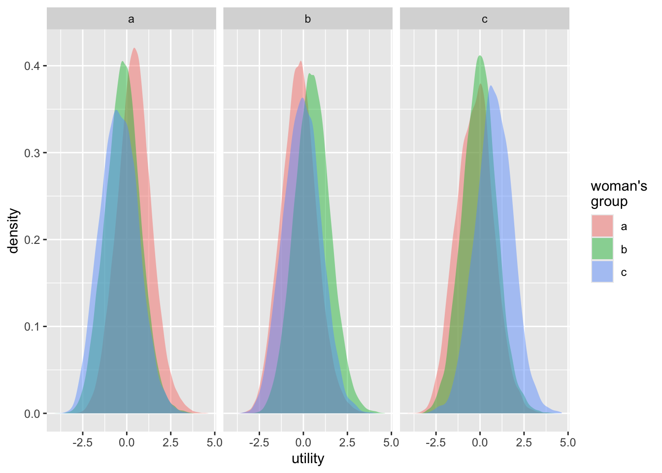
Plotting the distribution of utilities by group, shows, that utilities are higher for within group pairings, but with substantial heterogeneity and distributional overlap, as intended.

ggplot(data = union_utils, aes(x = utility, fill = group_woman)) +
  geom_density(alpha = 0.45, color = NA) +
  facet_wrap(~group_man) +
  labs(fill = "woman's\ngroup")

Simulated match utilities by man and woman’s group membership.

Tranforming utilities into unions

I use the the Gale-Shapley algorithm implemented in the matchingR package to transform the complete set of utilities into one-to-one dyadic matches. The package expects matrices of proposer utilities and reviewer utilities, where I treat the men as proposers and the women as reviewers. The proposer matrix contains the utilities men (in columns) would obtain from being matched with a given woman (in rows). The reviewer matrix contains the utilities the women (now in columns) would obtain from being matched with each man (in rows). In our case, we calculate a single utility for each union, and men’s and women’s matrices are transposes of each other. But in principle these matrices could differ more substantially in their elements. For example, the utility function that men use to evaluate women could differ from the function that women use to evaluate men. That’s a wrinkle to consider in a different post. In any case, the code to construct the matrices and make the matches is as follows:

men <- sort(filter(singles, sex == "man")$id)
women <- sort(filter(singles, sex == "woman")$id)
utility_matrix <- xtabs(utility ~ id_woman + id_man, data = union_utils)

unions <- matchingR::galeShapley.marriageMarket(
  proposerUtils = utility_matrix,
  reviewerUtils = t(utility_matrix)
)

matches <- tibble(
  id_man = as.integer(colnames(utility_matrix)),
  id_woman = as.integer(rownames(utility_matrix)[as.integer(unions$proposals)]),
  matched = TRUE
)

union_utils <-
  union_utils |>
  left_join(matches) |>
  mutate(matched = if_else(is.na(matched), FALSE, TRUE))

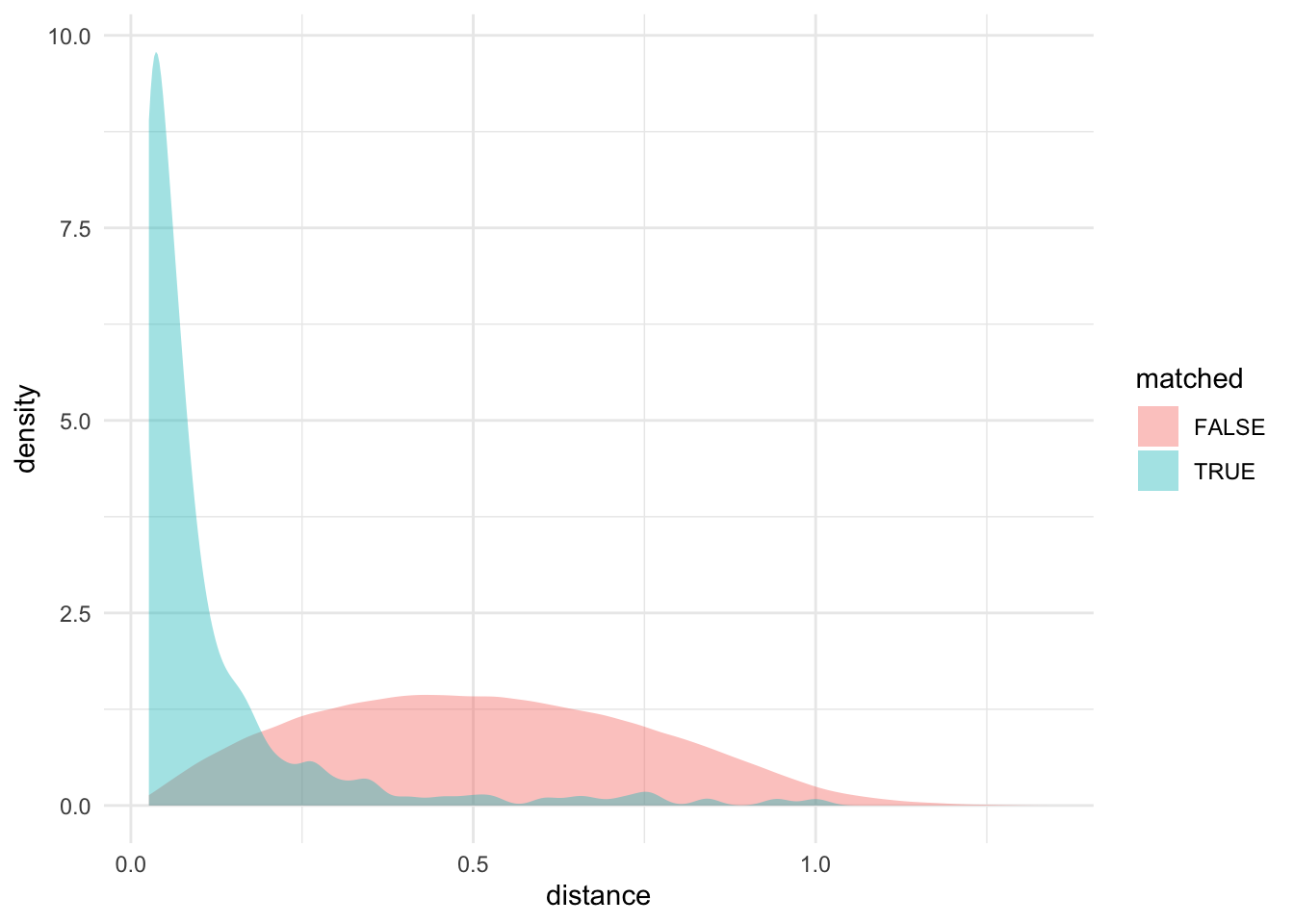
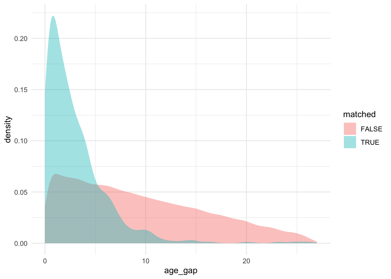
A quick glance suggests that the final matches align with what might be expected based on the utility functions used for simulation: The simulated matches are closer together in distance and age, and are more likely to share group membership, compared to the non-matches.

union_utils |>
  group_by(matched) |>
  summarize(across(c(distance, age_gap, same_group), ~ mean(.x)))

# A tibble: 2 × 4
  matched distance age_gap same_group
  <lgl>      <dbl>   <dbl>      <dbl>
1 FALSE      0.510    9.42      0.459
2 TRUE       0.115    3.01      0.748

And we can graphically compare the full distributions of distance and age gaps for matches vs. non-matches, once again confirming that things have worked as intended.

ggplot(data = union_utils, aes(x = distance, fill = matched)) +
  geom_density(alpha = 0.4, color = NA) +
  theme_minimal()

Distance to opposite sex in matched vs. non-matched pairs

ggplot(data = union_utils, aes(x = age_gap, fill = matched)) +
  geom_density(alpha = 0.4, color = NA) +
  theme_minimal()

Absolute age difference from opposite sex in matched vs. non-matched pairs

A reusable data generating function

For convenience, a data generating function can be wrapped around sub-functions that create actors, positions, position assignments, and matches. The main function, simulate_marriage_market(), returns a list containing the assigned singles, the realized matches, a lean exploded man-woman pair data set with matching utilities, and relevant input parameters. I produce the fully exploded pair utilities because they are useful for the modeling that I cover in the next post.

rbeta_scaled <- function(n, mean, precision, min_value = 0, max_value = 1) {
  scaled_mean <- (mean - min_value) / (max_value - min_value)
  shape1 <- scaled_mean * precision
  shape2 <- (1 - scaled_mean) * precision
  min_value + (max_value - min_value) * rbeta(n, shape1, shape2)
}

make_locations <- function(n, relax = 1.2) {
  dim <- ceiling(relax * sqrt(n))
  expand_grid(
    x = (seq_len(dim) - .5) / dim,
    y = (seq_len(dim) - .5) / dim
  ) |>
    arrange(x, y) |>
    mutate(id_location = row_number()) |>
    select(id_location, x, y)
}

make_actors <- function(
  n,
  groups,
  group_shares,
  age_mean,
  age_min,
  age_max,
  age_concentration
) {
  G <- length(groups)
  group_shares <- group_shares / sum(group_shares)
  group_counts <- as.integer(n * group_shares)
  group_counts[G] <- n - sum(group_counts[-G])

  tibble(group = groups, age_mean, group_counts) |>
    reframe(
      age = rbeta_scaled(
        group_counts,
        age_mean,
        precision = age_concentration,
        min_value = age_min,
        max_value = age_max
      ),
      .by = c(group, age_mean)
    ) |>
    mutate(id = row_number()) |>
    group_by(group) |>
    mutate(sex = if_else(as.logical(row_number() %% 2), "man", "woman")) |>
    select(id, sex, group, age)
}

d2 <- function(x1, y1, x2, y2) {
  sqrt((x1 - x2)^2 + (y1 - y2)^2)
}

locate_actors <- function(
  actors,
  locations,
  poles,
  params
) {
  utilities <- actors |>
    select(id, group, age) |>
    crossing(locations) |>
    left_join(poles, by = c("group" = "pole")) |>
    mutate(
      x_youth = poles[poles$pole == "youth", ]$x_pole,
      y_youth = poles[poles$pole == "youth", ]$y_pole,
      scale_youth = (mean(age) - age) / sd(age),
      group_distance = log(d2(x, y, x_pole, y_pole) + 0.01),
      youth_distance = log(d2(x, y, x_youth, y_youth) + 0.01),
      utility = params$group *
        group_distance +
        params$youth * scale_youth * youth_distance
    ) |>
    ungroup() |>
    mutate(
      utility = utility +
        params$noise * rnorm(n(), mean = 0, sd = sd(utility))
    ) |>
    arrange(desc(utility))

  assigned_actors <- integer()
  assigned_locations <- integer()
  assignments <- vector("list", nrow(actors))
  n_assigned <- 0L

  for (r in seq_len(nrow(utilities))) {
    option <- utilities[r, ]
    if (
      option$id %in%
        assigned_actors ||
        option$id_location %in% assigned_locations
    ) {
      next
    }
    n_assigned <- n_assigned + 1L
    assignments[[n_assigned]] <- option |>
      select(id, id_location)
    assigned_actors <- c(assigned_actors, option$id)
    assigned_locations <- c(assigned_locations, option$id_location)
    if (n_assigned == nrow(actors)) {
      break
    }
  }

  actors |>
    select(id, sex, group, age) |>
    left_join(bind_rows(assignments), by = "id") |>
    left_join(locations, by = "id_location") |>
    select(-id_location)
}

make_union_utilities <- function(singles, params) {
  cross_join(
    singles |> filter(sex == "man") |> rename_with(\(x) paste0(x, "_man")),
    singles |> filter(sex == "woman") |> rename_with(\(x) paste0(x, "_woman"))
  ) |>
    mutate(
      age_gap = abs(age_man - age_woman),
      distance = d2(x_man, y_man, x_woman, y_woman),
      same_group = 1L * (group_man == group_woman),
      utility = params$same_group *
        same_group +
        params$age_gap * age_gap +
        params$distance * log(distance + 0.01),
      utility = utility + params$noise * rnorm(n(), mean = 0, sd = sd(utility))
    ) |>
    ungroup() |>
    arrange(id_man, id_woman)
}

make_unions <- function(union_utils) {
  utility_matrix <- xtabs(utility ~ id_woman + id_man, data = union_utils)

  unions <- matchingR::galeShapley.marriageMarket(
    proposerUtils = utility_matrix,
    reviewerUtils = t(utility_matrix)
  )

  tibble(
    id_man = as.integer(colnames(utility_matrix)),
    id_woman = as.integer(rownames(utility_matrix)[as.integer(
      unions$proposals
    )]),
    matched = TRUE
  )
}

simulate_marriage_market <- function(
  seed = 543,
  n = 1000,
  groups = c("a", "b", "c"),
  group_shares = c(60, 30, 10),
  age_mean = c(35, 30, 25),
  age_min = 18,
  age_max = 45,
  age_concentration = 2,
  location_relax = 1.2,
  location_poles = tibble(
    pole = c("a", "b", "c", "youth"),
    x_pole = c(0.5, 0.25, 0.75, 0.5),
    y_pole = c(0.75, 0.25, 0.25, 0.5)
  ),
  location_params = list(group = -1, youth = -1, noise = 3),
  partner_params = list(
    same_group = 0.5,
    age_gap = -0.1,
    distance = -1,
    noise = 0.5
  )
) {
  set.seed(seed)

  actors <- make_actors(
    n = n,
    groups = groups,
    group_shares = group_shares,
    age_mean = age_mean,
    age_min = age_min,
    age_max = age_max,
    age_concentration = age_concentration
  )
  locations <- make_locations(n, relax = location_relax)
  singles <- locate_actors(
    actors = actors,
    locations = locations,
    poles = location_poles,
    params = location_params
  )

  union_utils <- make_union_utilities(singles, params = partner_params)
  matches <- make_unions(union_utils)

  list(
    singles = singles,
    matches = matches |>
      select(id_man, id_woman),
    utilities = union_utils |>
      select(id_man, id_woman, utility),
    parameters = list(
      location = location_params,
      partner = partner_params,
      seed = seed,
      n = n,
      groups = groups,
      group_shares = group_shares,
      age_mean = age_mean,
      age_min = age_min,
      age_max = age_max,
      age_concentration = age_concentration,
      location_relax = location_relax,
      location_poles = location_poles
    )
  )
}

As a quick check, I call the wrapper with a different set of assumptions and summarize the resulting matches. Specifically, I narrow the differences in group sizes, include stronger group clustering, reverse the age clustering effect, reduce the location assignment noise, and specify stronger preferences for same-group and same-age partners.

scenario_E <- simulate_marriage_market(
  seed = 678,
  n = 600,
  group_shares = c(50, 30, 20),
  age_mean = c(35, 30, 25),
  location_params = list(group = -1, youth = 1, noise = 0.2),
  partner_params = list(
    same_group = 2,
    age_gap = -0.2,
    distance = -0.5,
    noise = 0.5
  )
)

This yields the following distribution of singles:

ggplot(scenario_E$singles, aes(x, y, color = group, shape = sex, size = age)) +
  geom_point(alpha = 0.9) +
  coord_equal() +
  scale_color_manual(values = group_colors) +
  labs(
    x = "Spatial coordinate x",
    y = "Spatial coordinate y",
    color = "Group",
    shape = "Sex",
    size = "Age"
  ) +
  theme_void(base_size = 12) +
  theme(plot.margin = margin(2, 2, 2, 2))

Example marriage market generated by wrapper function.

And the following associations between being matched, utility, and utility ranks:

scenario_E$utilities |>
  left_join(
    scenario_E$matches |> mutate(matched = TRUE),
    by = c("id_man", "id_woman")
  ) |>
  mutate(matched = if_else(is.na(matched), FALSE, matched)) |>
  group_by(id_man) |>
  mutate(rank_woman = rank(desc(utility))) |>
  group_by(id_woman) |>
  mutate(rank_man = rank(desc(utility))) |>
  group_by(matched) |>
  summarize(across(c(utility, rank_woman, rank_man), mean))

# A tibble: 2 × 4
  matched utility rank_woman rank_man
  <lgl>     <dbl>      <dbl>    <dbl>
1 FALSE    -0.746     151.     151.  
2 TRUE      4.13        6.34     6.63

References

Breen, Richard. 1994. “Individual Level Models for Mobility Tables and Other Cross-Classifications.” Sociological Methods & Research 23 (2): 147–73. https://doi.org/10.1177/0049124194023002001.

Gullickson, Aaron. 2021. “A Counterfactual Choice Approach to the Study of Partner Selection.” Demographic Research 44: 513–36. https://doi.org/10.4054/DemRes.2021.44.22.

Haandrikman, Karen, and Leo J. G. van Wissen. 2012. “Explaining the Flight of Cupid’s Arrow: A Spatial Random Utility Model of Partner Choice.” European Journal of Population 28 (4): 417–39. http://www.jstor.org/stable/23274970.

Lindmarker, Jesper, and Benjamin F. Jarvis. 2025. “However Far Away? The Spatial Contingencies of Assortative Mating.” SocArXiv. https://doi.org/10.31235/osf.io/4tq8z_v1.

Logan, John A. 1983. “A Multivariate Model for Mobility Tables.” American Journal of Sociology 89 (2): 324–49. http://www.jstor.org/stable/2779144.

McFadden, Daniel. 1974. “Conditional Logit Analysis of Qualitative Choice Behaviour.” In Frontiers in Econometrics, edited by Paul Zarembka, 105–42. Economic Theory and Mathematical Economics. New York: Academic Press. http://elsa.berkeley.edu/pub/reprints/mcfadden/zarembka.pdf.

Footnotes

1. Confusingly, this is also sometimes referred to as the multinomial logistic regression model. In fact, the conditional logit model nests what sociologists and political scientists often call the multinomial model.